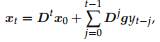
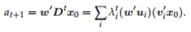
Студопедия — Stability and the Parameter Space
Студопедия Главная Случайная страница Обратная связь

Разделы: Автомобили Астрономия Биология География Дом и сад Другие языки Другое Информатика История Культура Литература Логика Математика Медицина Металлургия Механика Образование Охрана труда Педагогика Политика Право Психология Религия Риторика Социология Спорт Строительство Технология Туризм Физика Философия Финансы Химия Черчение Экология Экономика Электроника

Stability and the Parameter Space


In Chap.3, we found (p. 36) that, for linear models of the form (10.1), we could write the state vector as


where D = F − gw is the discount matrix. So for initial conditions to have a negligible effect on future states, we need Dt to converge to zero. There-
fore, we require D to have all eigenvalues inside the unit circle. We call this condition stability (following Hannan and Deistler 1988, p. 48).

Definition 10.3. The model (10.1) is said to be stable if all eigenvalues of D =

F − gw lie inside the unit circle.

Stability is a desirable property of a time series model because we want models where the distant past has a negligible effect on the present state.
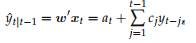
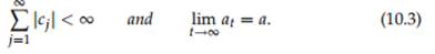
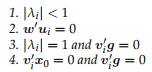
In Chap. 3, we also found that


where at = w Dt1x0 and cj = w Dj1g. Thus, the forecast is a linear func-
tion of the past observations and the seed state vector. This result shows that
for a model to be stable, we require the weaker forecastability condition:

Definition 10.4. The model (10.1) is forecastable if


Obviously, any model that is stable is also forecastable.


10.2 Stability and the Parameter Space 153

On the other hand, it is possible for a model to have a unit eigenvalue for D, but to satisfy the forecastability condition (10.3). In other words, an unstable model can still produce stable forecasts provided the eigenvalues which cause the instability have no effect on the forecasts. This arises because D may have unit eigenvalues where w is orthogonal to the eigenvectors corresponding to the unit eigenvalues.

To avoid complications, we will assume that all the eigenvalues are dis-
tinct. In this case, we can write the eigendecomposition of D as D = U ΛV, where the columns of U are the eigenvectors of D, Λ is a diagonal matrix containing the eigenvalues of D, and V = U1. Then


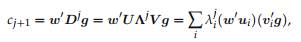
where ui is a column of U (a right eigenvector) and vi is a row of V (a left eigenvector). By inspection, we see that the sequence converges to zero pro-
vided either |λi | < 1, wui = 0 or vig=0,foreachi.Further,thesequence only converges under these conditions. Similarly,


In this case, the sequence converges to a constant if and only if either |λi | ≤
1, wui = 0 or vix0 = 0, for each i. Thus, we can restate forecastability as
follows.

Theorem 10.2. Let λi denote an eigenvalue of D = F − gw, and let ui be the
corresponding right eigenvector and vi the corresponding left eigenvector. Then the
model (10.1) is forecastable if and only if, for each i, at least one of the following four
conditions is met
:


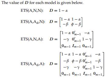
The concept of forecastability was noted by Sweet (1985) and Lawton
(1998) for ETS(A,A,A) (additive Holt-Winters) forecasts, although neither
author used a stochastic model as we do here. The phenomenon was also
observed by Snyder and Forbes (2003) in connection with the ETS(A,A,A)
model. The first general definition of this property was given by Hyndman
et al. (2008).

We now establish stability and forecastability conditions for each of the linear models. For the damped models, we assume that φ is a fixed damp-
ing parameter between 0 and 1, and we consider the values of the other parameters that would lead to a stable model.


154 10 Some Properties of Linear Models


Again, for ETS(A,A,N) and ETS(A,A,A), the corresponding result is obtained from ETS(A,Ad,N) and ETS(A,Ad,A) by setting φ = 1.


The stability conditions for models without seasonality (i.e., ETS(A,N,N),
ETS(A,A,N)and ETS(A,Ad,N)) are summarized in Table 10.1. These are given


10.2 Stability and the Parameter Space 155


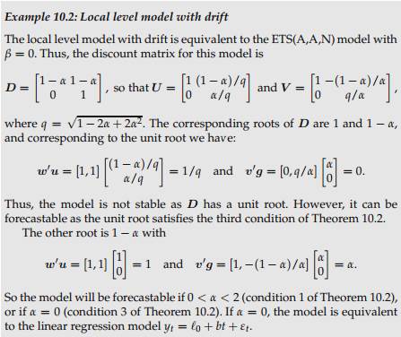
Fig. 10.1. Parameter spaces for model ETS(A,Ad,N). The right hand graph shows the
region for model ETS(A,A,N) (when φ = 1). In each case, the light-shaded regions rep-
resent the stability regions; the dark-shaded regions are the usual regions constructed
by restricting each parameter in the conventional parameterization to lie between 0
and 1.


in McClain and Thomas (1973) for the ETS(A,A,N) model; results for the
ETS(A,Ad,N) and ETS(A,N,N) models are obtained in a similar way. To
visualize these regions, we have plotted them in Fig. 10.1. The light-shaded
regions represent the stability regions; the dark-shaded regions are the usual
regions defined by 0 < β < α < 1. Note that the usual parameter region
is entirely within the stability region in each case. Therefore non-seasonal
models obtained using the usual constraints are always stable (and always
forecastable).


Дата добавления: 2015-09-07; просмотров: 447. Нарушение авторских прав; Мы поможем в написании вашей работы!


Композиция из абстрактных геометрических фигур Данная композиция состоит из линий, штриховки, абстрактных геометрических форм...

Важнейшие способы обработки и анализа рядов динамики Не во всех случаях эмпирические данные рядов динамики позволяют определить тенденцию изменения явления во времени...

ТЕОРЕТИЧЕСКАЯ МЕХАНИКА Статика является частью теоретической механики, изучающей условия, при ко­торых тело находится под действием заданной системы сил...

Теория усилителей. Схема Основная масса современных аналоговых и аналого-цифровых электронных устройств выполняется на специализированных микросхемах...

Что такое пропорции? Это соотношение частей целого между собой. Что может являться частями в образе или в луке...

Растягивание костей и хрящей. Данные способы применимы в случае закрытых зон роста. Врачи-хирурги выяснили...

ФАКТОРЫ, ВЛИЯЮЩИЕ НА ИЗНОС ДЕТАЛЕЙ, И МЕТОДЫ СНИЖЕНИИ СКОРОСТИ ИЗНАШИВАНИЯ Кроме названных причин разрушений и износов, знание которых можно использовать в системе технического обслуживания и ремонта машин для повышения их долговечности, немаловажное значение имеют знания о причинах разрушения деталей в результате старения...

Тема 5. Анализ количественного и качественного состава персонала Персонал является одним из важнейших факторов в организации. Его состояние и эффективное использование прямо влияет на конечные результаты хозяйственной деятельности организации.

Билет №7 (1 вопрос) Язык как средство общения и форма существования национальной культуры. Русский литературный язык как нормированная и обработанная форма общенародного языка Важнейшая функция языка - коммуникативная функция, т.е. функция общения Язык представлен в двух своих разновидностях...

Патристика и схоластика как этап в средневековой философии Основной задачей теологии является толкование Священного писания, доказательство существования Бога и формулировка догматов Церкви...

Studopedia.info - Студопедия - 2014-2024 год . (0.012 сек.) русская версия | украинская версия